XLOOKUP Return Multiple Columns at Once in Excel (One Formula That Spills)
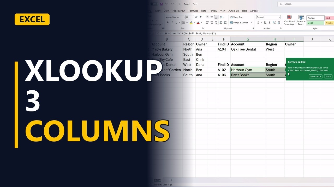
You do not need three XLOOKUPs to pull three columns. Make the return range wider and one XLOOKUP spills the account name, region and owner into the cells beside it. See the old way, the one-formula way, and the one thing never to do.
Try it yourself
Copy these tables into a blank sheet, then follow the steps below.
Paste at cell A1:
| ID | Account | Region | Owner |
|---|---|---|---|
| A101 | Maple Bakery | North | Ana |
| A102 | Harbour Gym | South | Ben |
| A103 | Blue Sky Cafe | East | Chris |
| A104 | Oak Tree Dental | West | Dana |
| A105 | Green Leaf Garden | North | Ben |
| A106 | River Books | South | Ana |
Paste at cell F1:
| Find ID | Account | Region | Owner |
|---|---|---|---|
| A104 |
Paste at cell F5:
| Find ID | Account | Region | Owner |
|---|---|---|---|
| A102 | |||
| A105 |
Step by step
- XLOOKUP, 3 columns. You don't need 3 XLOOKUP formulas to pull 3 columns. One XLOOKUP can return several columns at once, and the results spill into the cells beside it.
- The account list. The account list is in A1:D7. Column A has the ID, column B the account name, column C the region and column D the owner.
- What we want. We want all 3 details for the ID typed in F2.
- The old way. The old way uses one XLOOKUP per column. In G2, =XLOOKUP(F2,$A$2:$A$7,$B$2:$B$7) finds the ID in column A and returns the account name from column B. In H2, a second formula returns the region from column C, and you would need a third one for the owner in column D. That is 3 formulas to write, and 3 to fix when the list moves.
G2
=XLOOKUP(F2,$A$2:$A$7,$B$2:$B$7)H2
=XLOOKUP(F2,$A$2:$A$7,$C$2:$C$7) - One formula. Now the one-formula way, in the lower block. In G6, type =XLOOKUP(F6,$A$2:$A$7,$B$2:$D$7). It searches the same ID column, but the return range is 3 columns wide, B to D. Press Enter and the results spill. The account name, region and owner fill G6:I6, all from the one formula in G6.
G6
=XLOOKUP(F6,$A$2:$A$7,$B$2:$D$7) - Fill down. Fill G6 down to G7 for the next ID in F7. The $ signs keep both ranges fixed, and the new row spills on its own into G7:I7.
- It stays live. Type A106 in F7, and all 3 answers in G7:I7 change at once.
F7
A106 - Never type in the spill. Don't type in the spilled cells, such as H6:I7. If you do, the formula shows #SPILL! until you clear those cells again.
- Mark the spill. Give the spill area G6:I7 a light green fill (#E2EFDA). It tells the team those cells are taken. The fill is only a signal. It doesn't lock the cells.
- One formula. Make the return range as wide as the columns you want, and XLOOKUP gives them all back in one go. One formula per row means less to maintain.
Common mistakes
- Typing in a spilled cell. If any cell the results need already has something in it, even a space, the formula shows #SPILL!. Clear that cell, or move the formula to a spot with enough empty cells to its right.
- Leaving out the $ signs before filling down. Without them, A2:A7 turns into A3:A8 in the next row, and the first account drops out of the search. Lock both ranges, like $A$2:$A$7 and $B$2:$D$7.
- Putting the formula inside an Excel Table. Tables don't allow spilled results, so the formula shows #SPILL!. Put the lookup in a normal range next to the Table, or use one XLOOKUP per column inside it.
- Ranges with different numbers of rows. The return range must have as many rows as the search range, like $A$2:$A$7 and $B$2:$D$7. If they don't match, XLOOKUP returns #VALUE!.
When a business analyst uses this
In a RAID log, each risk has an owner ID, and the owners' details sit in a separate list. One XLOOKUP whose return range covers name, team and email spills all 3 in beside each risk, so there is one formula per row to check before the review. Keep the log as a normal range, because spills don't work inside an Excel Table.
Questions people ask
Which Excel versions can return multiple columns with XLOOKUP?
You need Microsoft 365, Excel 2021 or later, or Excel for the web, because they have both XLOOKUP and spilled results. Excel 2019 and older have neither.
Why does my XLOOKUP show #SPILL!?
Usually a cell the results need is not empty (even a space counts), so clear it or move the formula. You also get #SPILL! if those cells are merged or the formula sits inside an Excel Table, so unmerge the cells or move the formula outside the Table.
Can I edit just one of the spilled cells?
No. Only the first cell, like G6, holds the formula. The other cells just show its results, so you change the formula in G6 and the whole spill updates.