How to Use XLOOKUP in Excel (Beginner Tutorial for Business Analysts)
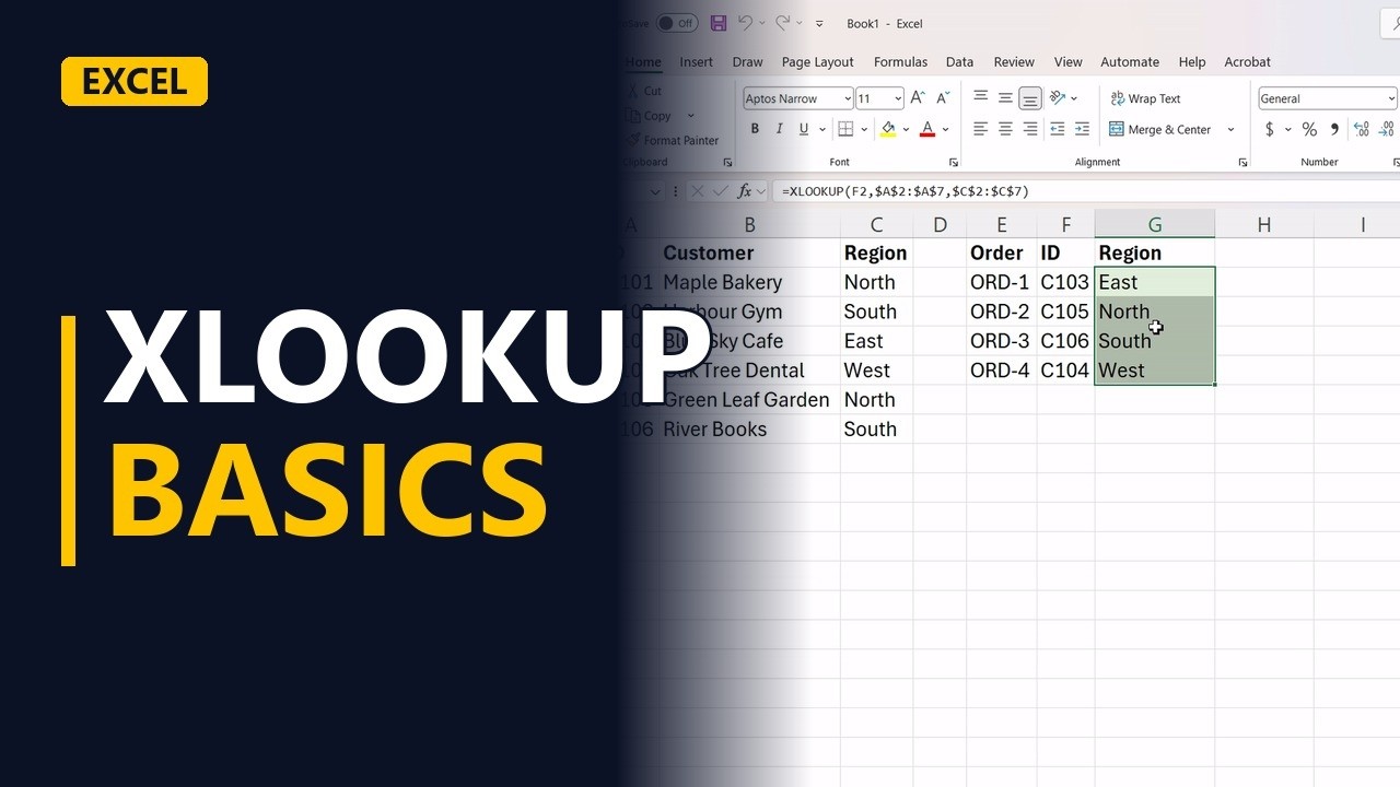
XLOOKUP finds a value in one list and returns the matching value from another. Learn the three parts of the formula by pulling each customer's region into an order list, then lock the ranges and fill it down.
Try it yourself
Copy these tables into a blank sheet, then follow the steps below.
Paste at cell A1:
| ID | Customer | Region |
|---|---|---|
| C101 | Maple Bakery | North |
| C102 | Harbour Gym | South |
| C103 | Blue Sky Cafe | East |
| C104 | Oak Tree Dental | West |
| C105 | Green Leaf Garden | North |
| C106 | River Books | South |
Paste at cell E1:
| Order | ID | Region |
|---|---|---|
| ORD-1 | C103 | |
| ORD-2 | C101 | |
| ORD-3 | C106 | |
| ORD-4 | C104 |
Step by step
- XLOOKUP basics. XLOOKUP finds a value in one list and returns the matching value from another. Here it pulls each customer's region into a list of orders.
- The customer list. The customer list sits in A1:C7. Each customer has an ID (column A), a name (column B) and a region (column C).
- The order list. The order list sits in E1:G5 and holds 4 orders. Each order only has the customer ID in column F. The region needs to appear in column G.
- What to find. Part 1 is what to find: the customer ID of the first order, in F2.
- Where to look. Part 2 is where to look: the ID column of the customer list, A2:A7.
- What to return. Part 3 is what to return: the region column, C2:C7. It covers the same rows as A2:A7.
- The formula. In G2, type =XLOOKUP(F2,$A$2:$A$7,$C$2:$C$7). The $ signs lock both lists, so they stay on the same rows when you copy the formula down.
G2
=XLOOKUP(F2,$A$2:$A$7,$C$2:$C$7) - The answer. G2 shows East. Excel found the ID from F2 in the customer list and returned the region on the same row.
- Fill down. Drag the fill handle from G2 down to G5. Every order now shows its customer's region.
- It stays live. The result stays live. Type C105 in F3 and the region in G3 changes to North by itself.
F3
C105 - Mark the formulas. Give the formula cells, G2:G5, a light green fill (#E2EFDA). It tells the team not to type over them.
- The 3 parts. XLOOKUP has 3 parts: what to find, where to look and what to return. Lock the 2 lists with $ signs before you fill down.
Common mistakes
- Leaving the ranges unlocked. Without the $ signs, A2:A7 shifts to A3:A8, A4:A9 and so on as you fill down, so lower rows miss customers and show #N/A. Write $A$2:$A$7 and $C$2:$C$7, or press F4 on each range.
- Ranges of different sizes. Where to look and what to return must cover the same rows, like A2:A7 and C2:C7. If they don't, XLOOKUP returns #VALUE!.
- An ID that isn't in the customer list. XLOOKUP returns #N/A when it finds no match. Add a fourth part for what to show instead, such as =XLOOKUP(F2,$A$2:$A$7,$C$2:$C$7,"Not found").
- IDs that look the same but don't match. A trailing space, or an ID stored as text in one list and as a number in the other, gives #N/A. Clean the IDs with TRIM and keep both lists the same type.
When a business analyst uses this
In a RAID log, each risk has an owner ID and the owners' names and teams sit on a stakeholder sheet. XLOOKUP pulls each owner's team into the log, so the workshop can see at a glance which team needs to act on each risk.
Questions people ask
How do I use XLOOKUP between 2 sheets?
Point where to look and what to return at the other sheet, for example =XLOOKUP(F2,Customers!$A$2:$A$7,Customers!$C$2:$C$7). You can also click across to the other sheet to select each range while typing the formula.
Can I use XLOOKUP in Excel 2016 or 2019?
No. XLOOKUP needs Microsoft 365, Excel 2021 or later, or Excel for the web. In Excel 2016 or 2019, use VLOOKUP or INDEX and MATCH instead.
Why use XLOOKUP instead of VLOOKUP?
XLOOKUP matches exactly by default, needs no column number and can return a column to the left of where it looks. You can also tell it what to show when nothing is found.