How to Make a Pivot Table in Excel (Beginner, in 5 Minutes)
A pivot table turns a long list into a summary in a few clicks. Build one from a small sales list: totals by region, split by product, a filter by month, and a chart, step by step in Excel.
Try it yourself
Copy this table into a blank sheet, then follow the steps below.
Paste at cell A1:
| Region | Product | Month | Sales |
|---|---|---|---|
| North | Laptop | Jan | 1,200 |
| North | Phone | Jan | 800 |
| South | Laptop | Jan | 950 |
| South | Tablet | Feb | 400 |
| East | Phone | Feb | 700 |
| East | Laptop | Feb | 1,100 |
| West | Tablet | Feb | 350 |
| West | Phone | Mar | 650 |
| North | Tablet | Mar | 500 |
| South | Phone | Mar | 900 |
| East | Tablet | Mar | 300 |
| West | Laptop | Mar | 1,000 |
Step by step
- Pivot table basics. A pivot table turns a long list into a short summary without any formulas. Here we build one from a small sales list in Excel.
- The data. The data is in A1:D13: one header row and 12 rows of sales. Each row has a Region, a Product, a Month and a Sales amount. There are no blank rows or columns, which is all a pivot table needs.
- Insert pivot table. Select A1:D13, then click Insert > PivotTable. Choose to put it on the same sheet, starting at F3, so you can see the data and the summary side by side.
- Rows. In the field list, drag Region into the Rows area. Excel lists each region once, however many times it appears in the data.
- Values. Drag Sales into the Values area. Each region now shows its total sales, with a grand total at the bottom. Here the totals use the #,##0 number format, so they're easier to read.
- Columns. Drag Product into the Columns area. Each region's total is now split into Laptop, Phone and Tablet, with a total for each product.
- Filters. Drag Month into the Filters area. A drop-down appears above the pivot table, so you can show only January or only March in one click.
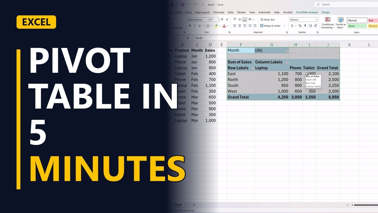
- Read the answer. Read the summary in F5:J9: laptops sell best in North and East. 12 rows of data have become one small table you can read in seconds.
- The four areas. Remember the four areas. Rows and Columns decide how the data is grouped. Values is what gets added up. Filters decide which rows are included.
- Pivot tips. A pivot table doesn't update by itself. When the data changes, right-click anywhere in the pivot table and choose Refresh.
Common mistakes
- Blank rows or blank headers in the data. A blank header stops Excel from making the pivot table, and a blank row can cut your data short. Give every column a header and remove empty rows before you insert it.
- Changing the data and expecting the totals to update. The pivot table keeps the old numbers until you refresh it. Right-click the pivot table and choose Refresh after every change.
- New rows added below the data are missing. The pivot table only reads its original source range, such as A1:D13. Turn the data into an Excel table with Ctrl+T before inserting the pivot table, so new rows are included when you refresh.
- Values shows Count instead of Sum. This happens when the Sales column has blanks or numbers stored as text. Fix the data, or click the field in Values, open Value Field Settings and choose Sum.
When a business analyst uses this
In a RAID log with one row per item, put Type in Rows, Status in Columns and ID in Values. The pivot table counts the open and closed risks, issues and dependencies for the weekly status report. If your IDs are numbers, set Value Field Settings to Count. Refresh it before each meeting.
Questions people ask
What is a pivot table in Excel?
It's a summary table that groups a long list and adds it up for you. Here it turns 12 rows of sales into total sales by region and product, with no formulas.
How do I make a pivot table with multiple columns?
Drag more than one field into the Columns or Rows area, and Excel nests the second one inside the first. You can also drag more than one field into Values to show several totals side by side.
Is it hard to make a pivot table in Excel?
No. If your data has one header row and no blank rows, it takes a few clicks: Insert > PivotTable, then drag fields into Rows, Columns, Values and Filters.