How to Use VLOOKUP in Excel (Step by Step for Beginners)
VLOOKUP finds a value in the first column of a table and returns a value from the same row. Learn its four parts by pulling each product's price into an order list, then lock the table with dollar signs and fill it down.
Try it yourself
Copy these tables into a blank sheet, then follow the steps below.
Paste at cell A1:
| ID | Product | Price |
|---|---|---|
| P101 | Desk Lamp | $35 |
| P102 | Office Chair | $149 |
| P103 | Notebook | $4 |
| P104 | Stapler | $12 |
| P105 | Monitor Stand | $45 |
| P106 | Wall Clock | $22 |
Paste at cell E1:
| Order | ID | Price |
|---|---|---|
| ORD-1 | P104 | |
| ORD-2 | P102 | |
| ORD-3 | P106 | |
| ORD-4 | P101 |
Step by step
- VLOOKUP basics. VLOOKUP finds things in a list. Here, a product list has the prices, but the orders only show the product ID. VLOOKUP pulls each price into the orders.
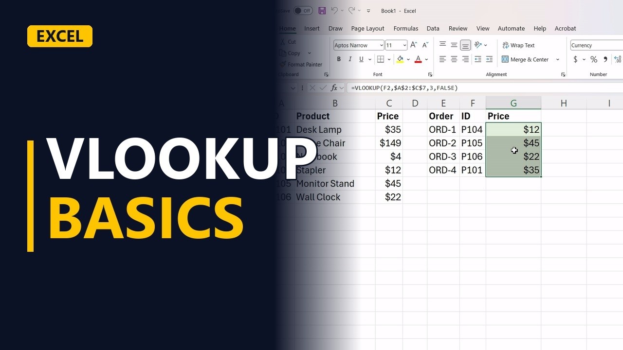
- The product list. The product list is in A1:C7. Each product has an ID in column A, a name in column B and a price in column C.
- The order list. The order list is in E1:G5 and has 4 orders. Each order only has the product ID, in column F. We want the price to show in column G.
- What to find. VLOOKUP has 4 parts. Part 1 is what to find. That's the product ID in F2.
- The table. Part 2 is the table to search, which is the whole product list, A2:C7. The ID must be in the first column of the table, because VLOOKUP only searches down the first column.
- Column number. Part 3 is the column number to return. Count from the left of the table: ID is 1, product is 2 and price is 3. So use 3.
- Exact match. Part 4 is FALSE, which means exact match. Always type it, or Excel may return the wrong price. Put the parts together in G2: =VLOOKUP(F2,$A$2:$C$7,3,FALSE).
G2
=VLOOKUP(F2,$A$2:$C$7,3,FALSE) - The answer. G2 shows $12. Excel found P104, the stapler, and returned its price from column 3.
- Lock the table. $A$2:$C$7 is an absolute reference. It locks the table, so it doesn't slide down when you copy the formula. Drag the fill handle from G2 down to G5.
- Every price. Every order now has its price: $149 for the chair, $22 for the clock and $35 for the lamp.
- It stays live. The formula stays live. Type P105 in F3 and the price in G3 changes to $45 by itself.
F3
P105 - Mark the formulas. Give the formula cells, G2:G5, a light green fill. Then the team knows not to type over them.
- The 4 parts. VLOOKUP has 4 parts: what to find, the table, the column number, and FALSE for an exact match. Lock the table with an absolute reference like $A$2:$C$7 before you fill down.
Common mistakes
- Leaving out FALSE. Without FALSE, VLOOKUP does an approximate match and can return the wrong price from a list that isn't sorted. Always end the formula with FALSE.
- Not locking the table before filling down. If you write A2:C7, the table moves down 1 row in each copied formula, so lower rows can miss products or show #N/A. Write $A$2:$C$7 so every copy searches the same table.
- The ID isn't in the first column of the table. VLOOKUP only searches down the first column of the range you give it. Start the table at the ID column. If the value you want is to the left of the ID, use XLOOKUP instead.
- Counting the column number from column A of the sheet. Count from the first column of the table, not the sheet. If the table starts at column B, then column D is column 3.
When a business analyst uses this
In a requirements log, each row has a stakeholder ID, and the names are on a Stakeholders sheet. =VLOOKUP(B2,Stakeholders!$A$2:$C$50,2,FALSE) pulls in each name. If the contact list changes, the log updates by itself, so you don't have to retype anything before a workshop or sign-off.
Questions people ask
What is VLOOKUP used for in Excel?
It looks up a value, like a product ID, in the first column of a table and returns a value from the same row, like the price. This saves you from copying values across by hand.
How do I use VLOOKUP from another sheet?
Put the sheet name and an exclamation mark before the table range, like =VLOOKUP(F2,Products!$A$2:$C$7,3,FALSE). The other 3 parts stay the same.
Can VLOOKUP return more than one column?
In Excel 2019 and older, each VLOOKUP returns 1 column, so copy it and change the column number (2 for the name, 3 for the price). In Microsoft 365 you can use {2,3} as the column number to get both columns at once.